surfview

npm

Interactive cortical surface rendering in the browser, built on Three.js

Installnpm install surfview three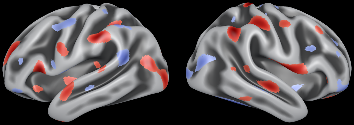

Lateral views of the left and right inflated fs_LR hemispheres on black, with a thresholded simulated statistic map: positive values in red, negative in blue, on grey sulcal shading

A simulated statistic map on the HCP fs_LR 32k inflated surfaces, rendered by surfview with the talk-dark preset: two exportPNG() exports side by side (in make-figures.mjs).

Classes NeuroSurfaceViewer · MultiLayerNeuroSurface · DataLayer · LabelLayer

Input GIFTI, FreeSurfer and ASCII PLY surfaces; scalar GIFTI maps

Layers Scalar, label, RGBA, outline, connectivity, volume-projection and temporal

Output PNG figures with colour keys, SVG atlas plates, portable report scenes

What it does

Surfaces load from GIFTI files, with folding shown on the inflated mesh

loadSurface() fetches a GIFTI, FreeSurfer or ASCII PLY surface, checks its coordinates and triangle indices, and returns a SurfaceGeometry. An inflated mesh has no folds to shade, so computeSulcalDepth() measures depth on the folded midthickness surface, whose vertices are the same; MultiLayerNeuroSurface draws it as a grey underlay, gyri light and sulci dark. NeuroSurfaceViewer owns the canvas and renders on demand, not in a permanent animation loop. You write no Three.js code; three is installed alongside as a peer dependency.

Each hemisphere has 32,492 vertices and 64,980 triangles; the left inflated GIFTI file is 710 KB. Unless the caller passes one, loadSurface() sets each surface’s hemisphere from the GIFTI metadata or, failing that, the file name; here it set left and right. computeSulcalDepth() runs on the CPU; one hemisphere took 120 ms in the headless Chromium that built this page. Compute it once, not per frame.

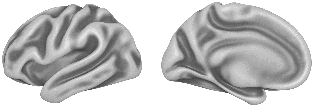
Lateral and medial views of the left inflated hemisphere in grey, with sulci darker than gyri

HCP fs_LR 32k template surfaces (Van Essen et al., 2012), from TemplateFlow (Ciric et al., 2022). Both views come from one viewer, turned with setAnatomicalView() and exported with exportPNG().

import {
  loadSurface, computeSulcalDepth, normalizeCurvature,
  MultiLayerNeuroSurface, NeuroSurfaceViewer
} from 'surfview';

// tf: URL of the TemplateFlow tpl-fsLR folder
// el: the page element that holds the canvas
const url = (h, kind) =>
  `${tf}/tpl-fsLR_den-32k_hemi-${h}_${kind}.surf.gii`;

const inflated = {}, folded = {}, depth = {};
for (const h of ['L', 'R']) {
  inflated[h] = await loadSurface(url(h, 'inflated'));
  folded[h] = await loadSurface(url(h, 'midthickness'));
  // Depth is measured on the folded surface; the inflated
  // mesh has the same vertices but no folds.
  depth[h] = normalizeCurvature(
    computeSulcalDepth(folded[h]));
}

const viewer = new NeuroSurfaceViewer(el, 800, 560,
  { preset: 'paper-light' });
const lh = new MultiLayerNeuroSurface(inflated.L, {
  curvature: depth.L,
  curvatureOptions: { brightness: 0.6, contrast: 0.36,
                      smoothness: 0.5 }
});
viewer.addSurface(lh, 'lh');
viewer.setAnatomicalView('lateral',
  { layout: 'single', surfaceId: 'lh', fit: true });

Thresholded maps, with the hidden interval on the colour key

DataLayer maps one value per vertex through a named colormap over range. Values inside threshold are not drawn, and neither are NaN values, which mark missing data. The shader draws the threshold boundary midway between drawn and hidden vertices, so at this mesh resolution the boundary follows the triangles.

exportPNG() renders the view at the requested pixel size and draws a colour key from the layer’s colormap, range and threshold: the hidden interval is hatched, and an arrow marks drawn values beyond the range.

2,796 of the left hemisphere’s 32,492 vertices lie in the HCP medial-wall mask and hold NaN, which the layer leaves undrawn; 4,041 of the remaining 29,696 (13.6%) have |z| > 1.5.

Lateral views of the left and right inflated hemispheres with a simulated z map thresholded at 1.5 in absolute value, and a colour key from -3 to 3 with the interval from -1.5 to 1.5 hatched

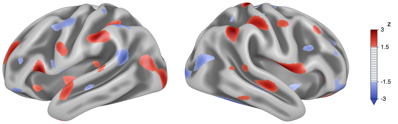
Simulated data: Gaussian noise at each vertex, averaged with its neighbours 60 times on the midthickness mesh and scaled to unit variance.

import { DataLayer } from 'surfview';

// Surfaces 'lh' (from 01) and 'rh' (built the same way)
// sim.L, sim.R: simulated z maps, one value per vertex
for (const [id, h] of [['lh', 'L'], ['rh', 'R']]) {
  viewer.addLayer(id, new DataLayer('z', sim[h], null,
    'coolwarm', {
      range: [-3, 3],
      threshold: [-1.5, 1.5]  // [-1.5, 1.5] not drawn
    }));
}
// The inflated meshes overlap at the midline: shift the
// left mesh 25 mm to the left and the right 25 mm right
viewer.separateHemispheres(50);
viewer.setAnatomicalView('lateral',
  { layout: 'single', surfaceId: 'rh', fit: true });

// A PNG at any size, with a colour key for layer 'z'
const png = viewer.exportPNG({
  width: 1200, height: 840, scaleBar: false,
  colorbarLayer: 'z', colorbarLabel: 'z', fontScale: 2
});

Atlases as label and outline layers

LabelLayer colours each vertex by its integer label from a table of label colours; labels missing from the table, here 0 on the medial wall, take defaultColor. OutlineLayer draws the boundaries between labels as lines along mesh edges. The curvature underlay stays at the bottom of the layer stack and outlines stay on top; the data and label layers between them can be reordered.

The file assigns the left hemisphere’s 200 parcels to 7 networks (Vis, SomMot, DorsAttn, SalVentAttn, Limbic, Cont, Default).

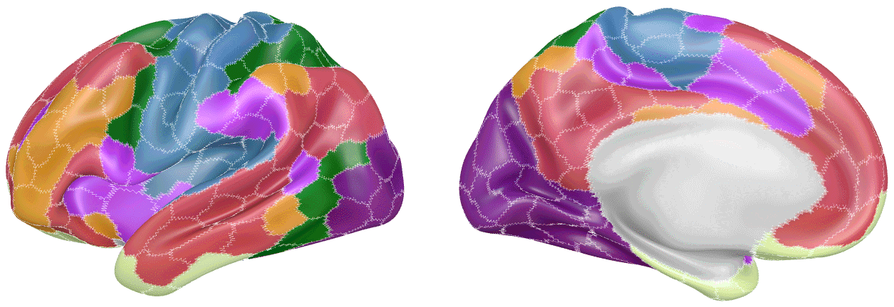
Lateral and medial views of the left inflated hemisphere coloured by the seven Yeo networks, with thin white lines between the Schaefer parcels; the medial wall is light grey

Schaefer–Yeo 400-parcel atlas (Schaefer et al., 2018) with the 7 networks of Yeo et al. (2011), left hemisphere on fs_LR 32k, in the atlas colours at 80% opacity.

import {
  LabelLayer, OutlineLayer, MultiLayerNeuroSurface,
  NeuroSurfaceViewer
} from 'surfview';

// Schaefer-400, 7 networks: left-hemisphere vertex labels
const res = await fetch(
  `${data}/schaefer/left-fslr32k-7networks.json`);
const atlas = await res.json();
const labels = Uint32Array.from(atlas.vertexLabels);

const viewer = new NeuroSurfaceViewer(el2, 800, 560,
  { preset: 'paper-light' });
const lh = new MultiLayerNeuroSurface(inflated.L, {
  curvature: depth.L,
  curvatureOptions: { brightness: 0.6, contrast: 0.36,
                      smoothness: 0.5 }
});
viewer.addSurface(lh, 'lh');

// Parcel colours; label 0 (medial wall) gets defaultColor
viewer.addLayer('lh', new LabelLayer('networks', {
  labels,
  labelDefs: atlas.parcels.map((p) =>
    ({ id: p.id, color: p.color, name: p.label })),
  defaultColor: '#d9d9d9',
  opacity: 0.8
}));
// Parcel boundaries, drawn as lines on top of the stack
viewer.addLayer('lh', new OutlineLayer('borders', {
  roiLabels: labels, color: 0xffffff, width: 1,
  opacity: 0.6
}));
viewer.setAnatomicalView('lateral',
  { layout: 'single', surfaceId: 'lh', fit: true });

Labelled atlas plates as vector graphics

buildAtlasPlate() projects an inflated surface and its vertex labels into a fixed lateral or medial view, traces the visible part of each parcel and places each name inside its parcel or, where the parcel is narrow, in the margin with a leader line. renderAtlasPlateSVG() writes the plate as SVG with one path per parcel and the names as text, without embedded images or scripts; AtlasPlateView shows the same plate in the page with clickable parcels.

The lateral plate shows 134 of the atlas’s 180 left-hemisphere parcels and names 67 of them, 16 through margin callouts; the other 67 visible parcels had too little area or no room for a label. The SVG is 801 KB.

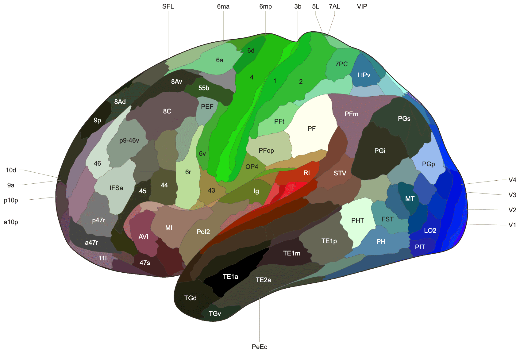
Flat lateral drawing of the left hemisphere divided into HCP-MMP1.0 parcels in their atlas colours, with area names such as V1, MT, 4, 3b, 44 and 45 inside the parcels or in the margins

HCP-MMP1.0 (Glasser et al., 2016), left hemisphere, in the atlas’s own colours. The SVG was rasterized for this page.

import {
  buildAtlasPlate, renderAtlasPlateSVG
} from 'surfview';

// HCP-MMP1.0 (Glasser et al., 2016): left-hemisphere labels
const res = await fetch(`${data}/glasser/left-fslr32k.json`);
const glasser = await res.json();

const plate = buildAtlasPlate({
  vertices: inflated.L.vertices,
  faces: inflated.L.faces,
  vertexLabels: glasser.vertexLabels,
  parcelData: glasser,
  hemisphere: 'left'
}, { view: 'lateral', width: 1200, height: 850,
     contourSmoothing: 4 });

// Standalone SVG: one path per parcel, labels as text
const colors = new Map(
  glasser.parcels.map((p) => [p.id, p.color]));
const svg = renderAtlasPlateSVG(plate, { colors });

Try it

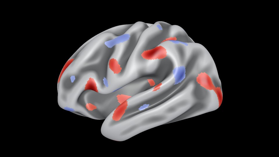
Still image of the viewer's starting view: the left inflated hemisphere from the side, with the simulated statistic map

View: |z| threshold 1.5

Both hemispheres of the HCP fs_LR 32k inflated surface (Van Essen et al., 2012; from TemplateFlow, Ciric et al., 2022), with the simulated map from 02 (|z| > 1.5 drawn, coolwarm from −3 to 3), in a NeuroSurfaceViewer with the talk-dark preset. It opens on the left hemisphere from the side; the buttons turn it to other views. The threshold slider calls viewer.updateLayer() on both hemispheres. The viewer is surfview 3.1.0’s browser build, surfview.embed.iife.js, which includes Three.js; nothing is fetched until the button is pressed.

Pressing the button fetches 3.2 MB: 1.3 MB of script and 1.9 MB of surface data.

Works with

neurosurf Its interactive htmlwidget bundles surfview’s browser build

three The WebGL renderer; a required peer dependency

Every figure on this page is rendered by surfview in headless Chromium by software/showcase/surfview/make-figures.mjs in the site’s source, and the code shown with each figure is the code that drew it.