neuroatlas

GitHub

Neuroimaging atlases and parcellations

Installpak::pak('bbuchsbaum/neuroatlas')

Left and right inflated cortical hemispheres in lateral and medial views, divided into 200 Schaefer parcels coloured by their seven resting-state networks, on a black background; the medial walls are dark grey

The Schaefer 200-parcel, 7-network atlas on the inflated fsaverage6 surface in the atlas’s network colours, drawn with plot_brain().

Atlases

17 loaders, including Schaefer, Glasser, HCPex, Brainnetome, Harvard-Oxford, Julich-Brain, ASEG

Representations Volume atlases on neuroim2 grids; surface atlases on fsaverage meshes

Lookup Region at an MNI coordinate, or every region within a radius

Parcel summaries Any function applied within each parcel, network or hemisphere

What it does

An atlas is a label volume with a metadata table

get_schaefer_atlas() returns an atlas object: a ClusteredNeuroVol of parcel ids together with the labels, hemisphere and network of each parcel. It downloads the Schaefer files on first use and caches them. outspace resamples the labels onto another grid with nearest-neighbour interpolation; here that is the 2 mm MNI152NLin6Asym template returned by get_template() from TemplateFlow. roi_metadata() returns one row per parcel.

list_atlases() lists the 17 atlas loaders registered in this version, with their representation (volume, surface or derived) and default template space.

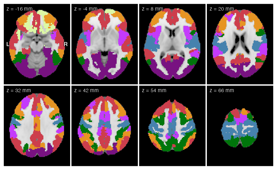
Eight axial slices of the MNI152NLin6Asym template with every cortical voxel coloured by its Schaefer network: visual in purple, somatomotor in blue, dorsal attention in green, salience/ventral attention in violet, limbic in pale yellow-green, control in orange, default in red

Network colours from the atlas’s own colour table: Vis · SomMot · DorsAttn · SalVentAttn · Limbic · Cont · Default.

library(neuroatlas)
library(neuroim2)

# MNI152NLin6Asym brain template at 2 mm, via TemplateFlow
tpl <- get_template("MNI152NLin6Asym", resolution = 2)

# Schaefer 2018: 200 parcels in 7 networks, with labels
# resampled onto the template grid (nearest neighbour)
sch <- get_schaefer_atlas(parcels = "200", networks = "7",
                          resolution = "2",
                          outspace = space(tpl))
meta <- roi_metadata(sch)  # one row per parcel

# Label each voxel with its parcel's network (1-7)
nets <- unique(meta$network)
lab  <- as.array(sch$atlas)  # parcel id per voxel, 0 = none
in_p <- lab > 0
net  <- NeuroVol(array(NA_real_, dim(lab)), space(tpl))
net[in_p] <- match(meta$network[match(lab[in_p], meta$id)],
                   nets)

# Draw in the atlas's own network colours: a palette with
# one flat step per integer label
first <- meta[match(nets, meta$network), ]
yeo <- rgb(first$color_r, first$color_g, first$color_b,
           maxColorValue = 255)
steps <- function(cols) {
  rep(cols, each = ceiling(256 / length(cols)))[1:256]
}
fig <- plot_overlay(tpl, net, ov_cmap = steps(yeo),
                    ov_range = c(0.5, 7.5), n_slices = 8,
                    ncol = 4, colorbar = FALSE)

Coordinates to region names

query_point() takes one coordinate or a matrix of coordinates in millimetres and returns a tibble with the region id, label, hemisphere and network at each point, one row per point and atlas for an exact lookup. Given a named list of atlases, it queries all of them; background voxels return NA. The ASEG subcortical atlas used here ships with the package.

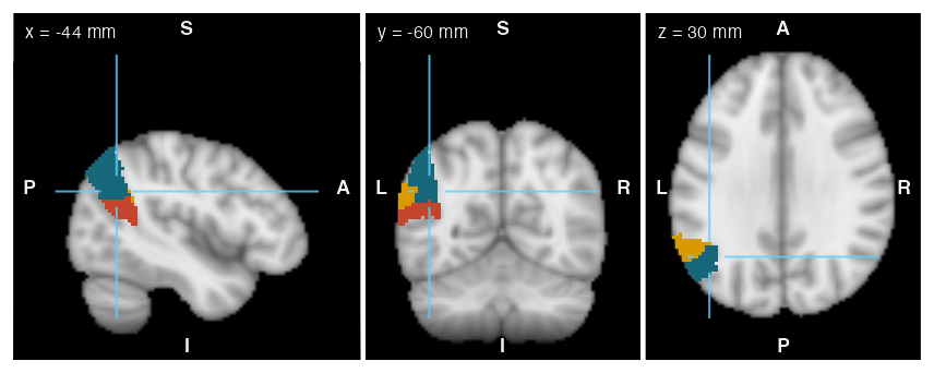
With radius = 8, the same call returns every parcel that has a labelled voxel within 8 mm of the point: 3 parcels here, LH_Default_Par_1, LH_Default_Par_4, LH_Default_Par_3. The figure shows these parcels in slices through point 1.

Sagittal, coronal and axial views through MNI coordinate (-44, -60, 30) in left inferior parietal cortex, with the three nearby Default-network parcels in coral, teal and gold; the crosshair lies in the teal parcel

Point	MNI	Schaefer	Network	ASEG
1	(-44, -60, 30)	`Par_4` (L)	Default	–
2	(40, 22, 40)	`PFCl_7` (R)	Cont	–
3	(-8, -56, 30)	`pCunPCC_2` (L)	Default	–
4	(-26, -22, -15)	–	–	`Hippocampus` (L)

Exact lookup (radius = 0) at four MNI152 coordinates, in mm. L and R give the hemisphere; a dash means the point is outside that atlas’s labels.

# Which region lies at each MNI coordinate (mm)? Query
# the Schaefer atlas and the bundled FreeSurfer ASEG.
pts <- rbind(c(-44, -60, 30), c(40, 22, 40),
             c(-8, -56, 30), c(-26, -22, -15))
hits <- query_point(pts, list(Schaefer = sch,
                              ASEG = get_aseg_atlas()))

# Every parcel with a voxel within 8 mm of point 1
near <- query_point(pts[1, ], sch, radius = 8)

nearby <- NeuroVol(array(NA_real_, dim(lab)), space(tpl))
for (k in seq_len(nrow(near))) {
  nearby[lab == near$id[k]] <- k
}
near_cols <- c("#c4452b", "#17677a", "#d99a00",
               "#7b3fa0", "#2e8b57", "#5a6f80")[1:nrow(near)]
fig <- plot_ortho(tpl, coord = pts[1, ], unit = "mm",
                  overlay = nearby,
                  ov_cmap = steps(near_cols),
                  ov_range = c(0.5, nrow(near) + 0.5),
                  colorbar = FALSE)

One value per parcel from any image on the atlas grid

reduce_atlas() applies a function, such as mean, to the voxels of each parcel and returns a tibble with one row per parcel (columns region and value); for a 4D NeuroVec the default is one row per time point and one column per parcel. The image must have the atlas’s dimensions. With level = "network" or "hemisphere", the function is applied again to the parcel values within each group.

The simulated map adds 0.5 to every voxel of the 46 Default-network parcels. The Default network mean is 0.50; the other six lie between -0.09 and 0.26 (vertical bars).

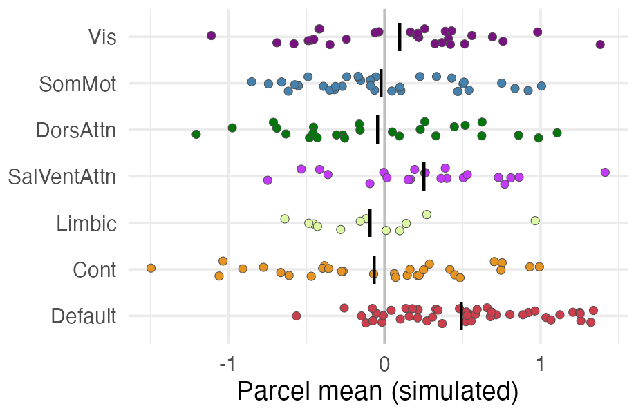
Dot plot of 200 parcel means grouped by the seven networks, each dot in its network colour, with a black bar at each network mean; the Default-network bar sits near 0.5 and the others near zero

Simulated data: smoothed Gaussian noise (12 mm FWHM, unit variance) with 0.5 added inside the Default network. Each dot is a parcel; bars are network means.

# Simulated statistic map: smoothed Gaussian noise in the
# parcels, plus 0.5 in every Default-network parcel
set.seed(3)
mask  <- NeuroVol(as.numeric(in_p), space(tpl))
noise <- NeuroVol(rnorm(length(lab)), space(tpl))
stat  <- gaussian_blur(noise, mask, fwhm = 12)
stat  <- stat / sd(stat[in_p])  # unit variance
dmn   <- lab %in% meta$id[meta$network == "Default"]
stat[dmn] <- stat[dmn] + 0.5

# Mean within each parcel: one row per parcel
pm <- reduce_atlas(sch, stat, mean)   # region, value
pm$network <- meta$network[match(pm$region,
                                 meta$label_full)]
# The same function over the parcel means of each network
nm <- reduce_atlas(sch, stat, mean, level = "network")

library(ggplot2)
names(yeo) <- nets
fig <- ggplot(pm, aes(value, factor(network, rev(nets)))) +
  geom_vline(xintercept = 0, colour = "grey75") +
  geom_jitter(aes(fill = network), height = 0.18,
              shape = 21, colour = "grey30", size = 2.2,
              stroke = 0.3) +
  geom_point(data = nm, shape = 124, size = 8) +
  scale_fill_manual(values = yeo, guide = "none") +
  labs(x = "Parcel mean (simulated)", y = NULL) +
  theme_minimal(base_size = 16)

Parcel values on the cortical surface

schaefer_surf() returns the same parcellation as a surface atlas: one label per vertex on the fsaverage6 geometry bundled with the package, with annotation files downloaded and cached on first use. align_parcel_values() matches a results table to the atlas by a key column and returns the values in atlas order; it stops on duplicate, unknown or missing parcels unless allow_partial = TRUE. plot_brain() draws them; static_backend = "cpu" rasterises the parcels over a sulcal-depth underlay without OpenGL or a browser.

The volume and surface versions of Schaefer-200 carry the same 200 ids and labels (checked at build time). Each fsaverage6 hemisphere has 40,962 vertices.

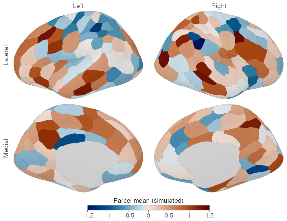
Lateral and medial views of both inflated hemispheres with each Schaefer parcel filled by its simulated mean on a blue-white-brown scale symmetric about zero; the medial wall is grey

The parcel means from feature 03 (simulated data), on a colour scale symmetric about zero.

# The same parcels on the fsaverage6 inflated surface
# (the annotation files are downloaded once, then cached)
surf <- schaefer_surf(parcels = 200, networks = 7,
                      space = "fsaverage6", surf = "inflated")

# Match the parcel table to the surface atlas by full
# region name; the result is in surf$ids order
vals <- align_parcel_values(surf, pm, value = value,
                            by = c(label_full = "region"))
lim <- c(-1, 1) * ceiling(10 * max(abs(vals))) / 10
fig <- plot_brain(surf, vals = vals, interactive = FALSE,
                  static_backend = "cpu", palette = "vik",
                  lim = lim, colorbar = "bottom",
                  colorbar_title = "Parcel mean (simulated)",
                  orientation_labels = FALSE)

Built on

neuroim2 Volumes, spaces and ROIs

Every figure on this page is drawn by software/showcase/neuroatlas/make-figures.R in the site’s source, and the code shown with each figure is the code that drew it.