Software

neurosurf

GitHub

Brain surface mesh reading and visualization

Installpak::pak('bbuchsbaum/neurosurf')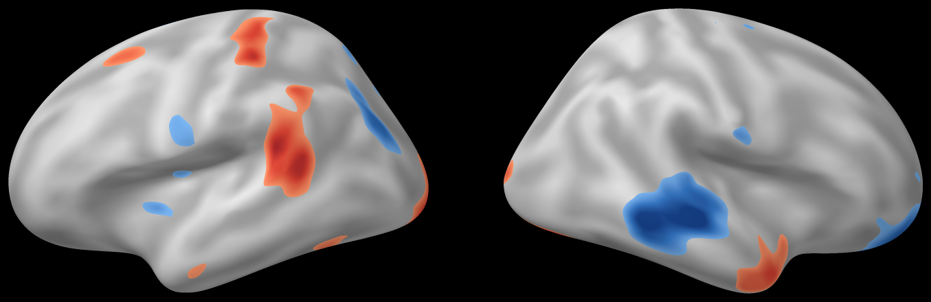

Documentation Source on GitHub

A simulated statistic map on the bundled inflated fsaverage surfaces, drawn with surface_figure() (in make-figures.R).

Classes SurfaceGeometry · NeuroSurface · NeuroSurfaceVector · LabeledNeuroSurface

Input / output FreeSurfer and GIFTI meshes; GIFTI, NIML and AFNI 1D vertex data

Static figures CPU rasterizer: PNG without OpenGL or a browser

Analysis on the mesh Volume projection, geodesic distance, smoothing, clusters, searchlights

What it does

01

Volumes are sampled through the cortical ribbon

vol_to_surf() samples a NeuroVol between matched white and pial surfaces and returns a NeuroSurface with one value per vertex. Here it reads the bundled Schaefer-200 atlas at five depths, from 10% to 90% of cortical thickness, by nearest voxel and keeps the most frequent label. The white, pial and inflated meshes share one vertex numbering, so render_surface_parcels() can draw the labels on the inflated surface.

Each hemisphere has 642 vertices. The projection recovers 100 of the atlas’s 100 left-hemisphere parcels and 100 of its 100 right-hemisphere parcels. 83 left and 90 right vertices get label 0 (outside every parcel), the most frequent value among their five depth samples; in the left hemisphere shown they are the grey medial wall and a few vertices elsewhere.

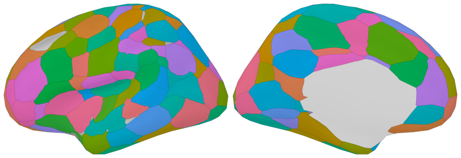
Parcel colours are arbitrary. The code treats the fsaverage surface coordinates and the atlas’s MNI152 coordinates as the same space, which they are only approximately.

library(neurosurf)
library(neuroim2)

# fsaverage meshes bundled with the package, resampled
# with AFNI MapIcosahedron (642 vertices per hemisphere)
white <- load_fsaverage_std8("white")
pial  <- load_fsaverage_std8("pial")
infl  <- load_fsaverage_std8("inflated")
curv  <- lapply(white, curvature)  # folding, for shading

# The Schaefer-200 atlas (MNI152, 1 mm) also ships with it
f <- list.files(system.file("extdata", package = "neurosurf"),
                pattern = "^Schaefer.*gz$", full.names = TRUE)
atlas <- read_vol(f)

# Most frequent label at five depths from white to pial
project <- function(h)
  vol_to_surf(white[[h]], pial[[h]], atlas,
              sampling = "thickness",
              depth = seq(0.1, 0.9, length.out = 5),
              interpolation = "nearest", aggregate = "mode")
labels <- lapply(c(lh = "lh", rh = "rh"), function(h)
  as.integer(values(project(h))))  # 0 = no atlas label

# Draw the labels on the inflated mesh (same vertices)
prep <- prepare_surface_parcels(infl$lh, labels$lh,
                                anatomy_metric = curv$lh)
set.seed(4)  # parcels 1-100 are the left hemisphere's
cols <- setNames(sample(hcl.colors(100, "Dark 3")), 1:100)
views <- lapply(c("lateral", "medial"), function(v)
  render_surface_parcels(prep, colors = cols, camera = v))

# Each panel is an RGBA raster; place them side by side
as_image <- function(p) magick::image_read(aperm(p$rgba, 3:1))
fig <- magick::image_append(do.call(c, lapply(views,
                                              as_image)))

02

All views share one threshold and colour scale

surface_figure() renders every hemisphere and view with the same threshold, limits and palette and returns a surface_figure object, which plot() draws and write_surface_figure() saves as PNG. The rasterizer runs on the CPU, so it needs neither OpenGL nor a browser. It interpolates values within each triangle before thresholding, so a threshold boundary can cross a triangle rather than follow its edges.

smooth() replaces each vertex value with the mean over the vertices within sigma mm along the surface; despite its name, sigma is a radius, not a Gaussian width.

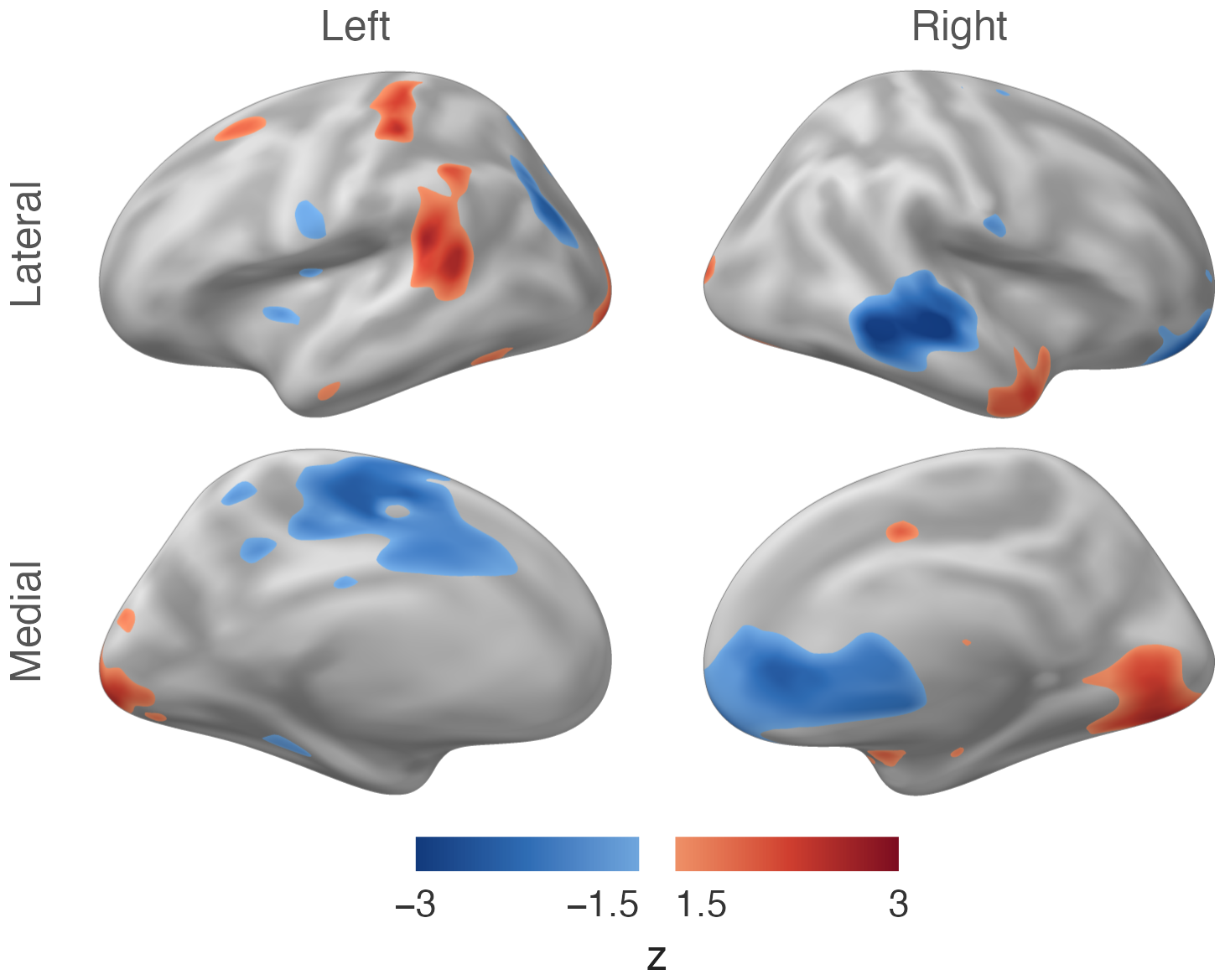
Simulated data: Gaussian noise averaged within 30 mm along the white surface, rescaled to unit variance and thresholded at |z| = 1.5.

# Simulated map: Gaussian noise at each vertex, averaged
# over a 30 mm geodesic radius on the white surface
set.seed(18)
sim <- lapply(white, function(g) {
  n  <- length(nodes(g))
  ns <- NeuroSurface(g, seq_len(n), data = rnorm(n))
  z  <- values(smooth(ns, sigma = 30))  # sigma: radius, mm
  (z - mean(z)) / sd(z)                 # unit variance
})

# Four views, one threshold, one colour scale
fig <- surface_figure(lh = infl$lh, rh = infl$rh,
                      values = sim, anatomy = curv,
                      threshold = 1.5, limits = c(-3, 3),
                      legend_title = "z")

03

Neighbourhoods measured along the cortex

geodesic_distances() returns shortest-path distances along the mesh edges (Dijkstra’s algorithm, with edge lengths in mm as weights) from source to target vertices. Teal marks vertices within 20 mm of a seed along the white surface; red marks vertices within 20 mm in a straight line but not along the surface, on the far side of a sulcus. On this 642-vertex mesh, edge paths zig-zag (overstating distance) and decimation flattens sulcal depth (understating it); use a full-resolution mesh for real analyses.

Of the 40 vertices within 20 mm of the seed in a straight line, 27 are 20 mm or more away along the surface, 18 of them 40 mm or more; the farthest is 114 mm away. SurfaceSearchlight(distance_type = "geodesic") builds its neighbourhoods from the same edge-path distances. With a 12 mm radius on this mesh, whose median edge is 10.2 mm long, it returns 642 searchlights of 2 to 9 vertices (mean 5.5).

Without distance_type, SurfaceSearchlight() uses straight-line distance.

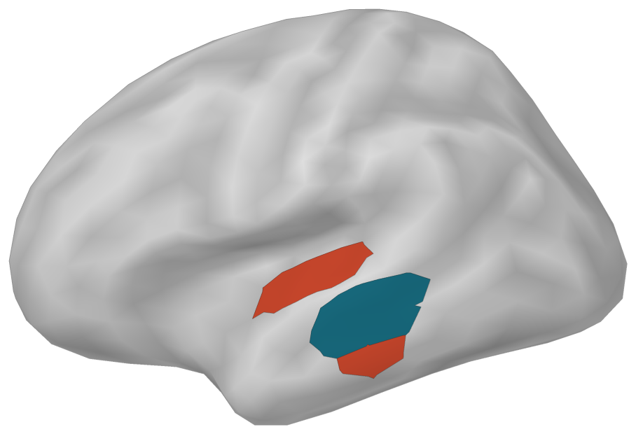
Distances are computed on the white surface and drawn on the inflated surface; the lateral view shows only some of the red vertices.

# Distance from one vertex in left lateral temporal
# cortex, along the white surface and in a straight line
seed <- 488
xyz  <- coords(white$lh)
geo  <- geodesic_distances(white$lh, seed,
                           targets = nodes(white$lh))
geo  <- as.vector(geo)
euc  <- sqrt(colSums((t(xyz) - xyz[seed, ])^2))

# 1: neither; 2: within 20 mm along the surface;
# 3: within 20 mm in a straight line only
r    <- 20
zone <- ifelse(geo < r, 2L, ifelse(euc < r, 3L, 1L))
prep <- prepare_surface_parcels(infl$lh, zone,
                                anatomy_metric = curv$lh)
fig  <- as_image(render_surface_parcels(prep,
          colors = c("2" = "#17677a", "3" = "#c4452b")))

# Searchlights defined by geodesic radius, one per vertex
sl <- SurfaceSearchlight(white$lh, radius = 12,
                         distance_type = "geodesic",
                         as_deflist = TRUE)

04

Cluster-extent thresholds on the mesh graph

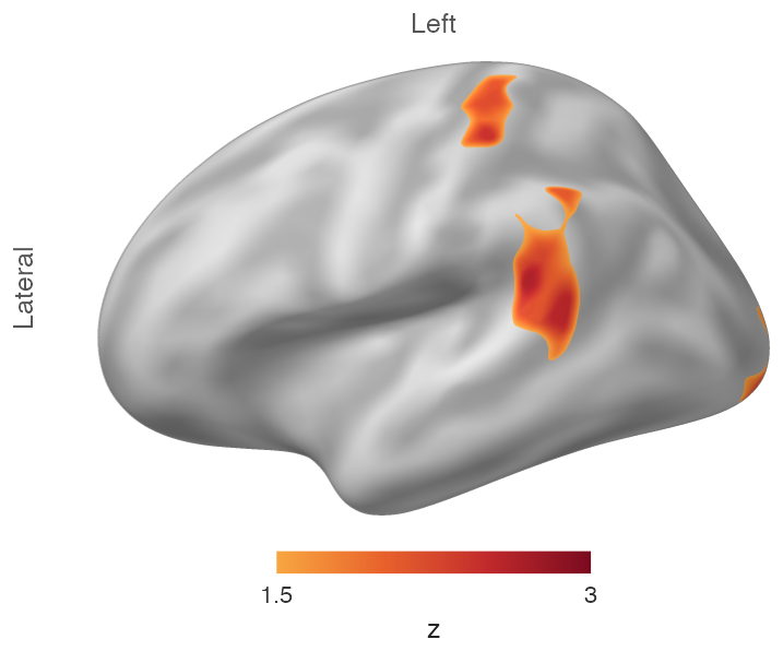
cluster_threshold() returns the input NeuroSurface with every vertex outside a component of at least size connected vertices set to 0. conn_comp() returns two NeuroSurface objects holding each vertex’s component index and component size. Both take a two-element threshold and keep vertices at or below the first value or at or above the second, so c(-Inf, 1.5) selects z ≥ 1.5.

The left hemisphere has 8 connected components at z ≥ 1.5; 3 of them have 5 or more vertices and survive.

Cluster	Vertices	Peak vertex	Peak (mm)	z
1	16	506	(-51, -43, 18)	2.66
2	11	302	(-44, -32, 53)	2.46
3	9	558	(-13, -96, -13)	2.46

The left hemisphere of the simulated map in 02, drawn with the positive-tail palette. Cluster 3 lies mostly on the medial surface, outside this view. Peaks are the peak vertex’s position on the fsaverage white surface.

# Cluster-extent threshold on the left hemisphere: keep
# components of 5 or more connected vertices with z >= 1.5
# (conn_comp and cluster_threshold keep values <= the
# lower bound or >= the upper bound)
lh_map <- NeuroSurface(white$lh, seq_along(sim$lh),
                       sim$lh)
kept   <- cluster_threshold(lh_map, threshold = c(-Inf, 1.5),
                            size = 5)

# Component labels and sizes, for the table
cc   <- conn_comp(kept, threshold = c(-Inf, 1.5))
comp <- values(cc$index)  # component id; 0 = not kept

fig <- surface_figure(lh = infl$lh, values = values(kept),
                      anatomy = curv$lh, views = "lateral",
                      threshold = 1.5, tail = "positive",
                      limits = c(1.5, 3), legend_title = "z")

Built on

neuroim2 Volumes read and sampled by vol_to_surf()

igraph The mesh graph behind distances and clusters

rgl Mesh storage and the interactive viewer

Every figure on this page is drawn by software/showcase/neurosurf/make-figures.R in the site’s source, and the code shown with each figure is the code that drew it.